KAMP Rotor Vibration Data
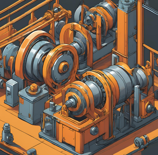
This post is about detecting bearing failure based on vibration values of a bearing mounted on a rotating machine.
Table of Contents
- Data Introduction
- Data Visualization with Machbase Neo
- Table Creation and Data Upload in Machbase Neo
- Experimental Methodology
- Experiment Code
- Experimental Results
1. Data Introduction
- DataHub Serial Number: 2024-2.
- Data Name: Rotating Machine Fault Type AI Dataset.
- Data Collection Methods: Collecting test data for various types of failures using the rotor testbed.
- Data Source: Link
- Raw data size and format: 73MB, CSV.
- Number of tags: 32.
| Tag | Description |
|---|---|
| g1_sensor1~4_normal | Normal state data from four sensors in Group 1. |
| g1_sensor1~4_type1 | Type1 state data from four sensors in Group 1. |
| g1_sensor1~4_type2 | Type2 state data from four sensors in Group 1. |
| g1_sensor1~4_type3 | Type3 state data from four sensors in Group 1. |
| g2_sensor1~4_normal | Normal state data from four sensors in Group 2. |
| g2_sensor1~4_type1 | Type1 state data from four sensors in Group 2. |
| g2_sensor1~4_type2 | Type2 state data from four sensors in Group 2. |
| g2_sensor1~4_type3 | Type3 state data from four sensors in Group 2. |
- State : 4.
| State | Description |
|---|---|
| Normal | Normal. |
| type1 | Disk rotational imbalance. |
| type2 | Support imbalance. |
| type3 | Type 1 + Type 2. |
- Sample Rate: 1000.
- Data Time Range: 2024-01-01 00:00:00 to 2024-01-01 00:02:19.
- Number of data records collected: 6,035,815.
- CSV data URL: https://data.yotahub.com/2024-2/datahub-2024-2-rotor.csv.gz
- Data Migration: KAMP Rotor Vibration Data Migration
2. Data Visualization with Machbase Neo
- Data visualization is possible through the Tag Analyzer in Machbase Neo.
- Select desired tag names and visualize them in various types of graphs.
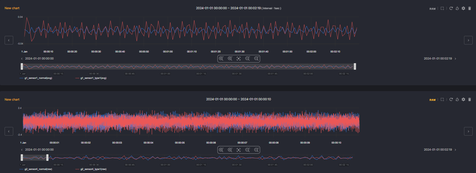
- Below, access the 2024-2 DataHub in real-time, select the desired tag names from the data of 32 tags, visualize them, and preview the data patterns.
DataHub Viewer
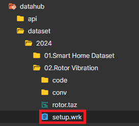
3. Table Creation and Data Upload in Machbase Neo
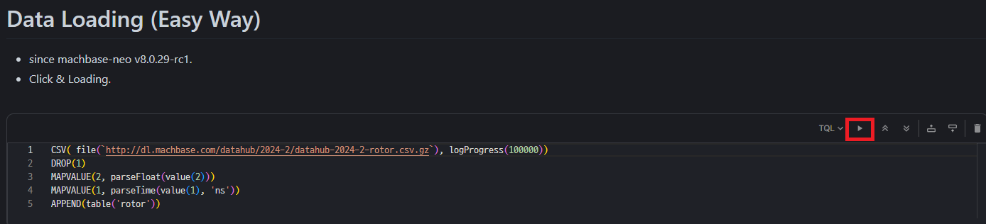
- In the DataHub directory, use setup.wrk located in the Rotor Vibration Dataset folder to create tables and load data, as illustrated in the image below.
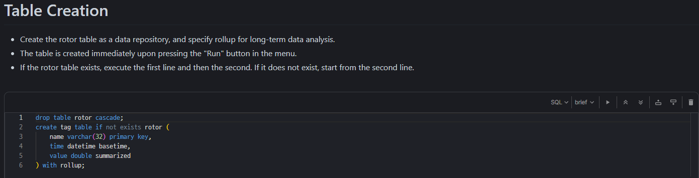
1) Table Creation
- The table is created immediately upon pressing the "Run" button in the menu.
- If the rotor table exists, execute the first line and then the second. If it does not exist, start from the second line.
2) Data Upload
- Loading tables in two different ways.
Method 1) Table loading method using TQL in Machbase Neo (since machbase-neo v8.0.29-rc1
-
Pros
- Machbase Neo loads as soon as you hit the launch button.
-
Cons
- Slower table loading speed compared to other method.
Method 2) Loading tables using commands
-
Pros
- Fast table loading speed.
-
Cons
- The table loading process is cumbersome.
- Run cmd window - Change machbase-neo path - Enter command in cmd window.
- If run the below script from the command shell, the data will be entered at high speed into the rotor table.
curl http://data.yotahub.com/2024-2/datahub-2024-2-rotor.csv.gz | machbase-neo shell import --input - --compress gzip --header --method append --timeformat ns rotor
- If specify a separate username and password, use the --user and --password options (if not sys/manager) and add the options as shown below.
curl http://data.yotahub.com/2024-2/datahub-2024-2-rotor.csv.gz | machbase-neo shell import --input - --compress gzip --header --method append --timeformat ns rotor --user USERNAME --password PASSWORD
4. Experimental Methodology
- Model Objective: Rotor condition classification.
- Tags Used: Group 1 (16 Tags).
- Model Configuration: ResNet 1d.
- Learning Method: Supervised Learning.
- Train: Model Training.
- Validation: Model validation.
- Test: Model Performance Evaluation.
- Model Optimizer: Adam.
- Model Loss Function: CrossEntropyLoss.
- Model Performance Metric: F1 Score.
- Data Loading Method
- Loading the Entire Dataset.
- Loading the Batch Dataset.
- Data Preprocessing
- Hanning Window.
- Fast Fourier Transform.
- MinMax Scaling.
5. Experiment Code
- Below is the code for each of the two ways to get data from the database.
- If all the data can be loaded and trained at once without causing memory errors, then method 1 is the fastest and simplest.
- If the data is too large, causing memory errors, then the batch loading method proposed in method 2 is the most efficient.
Method 1) Loading the Entire Dataset
- The code below is implemented in a way that loads all the data needed for training from the database all at once.
- It is exactly the same as loading all CSV files (The only difference is that the data is loaded from Machbase Neo).
- Pros
- Can use the same code that was previously utilizing CSVs (Only the loading process is different).
- Cons
- Unable to train if trainable data size exceeds memory size.
- The entire code can be run through 2.Rotor_General.ipynb.
Method 2) Loading the Batch Dataset
- Method for loading data from the Machbase Neo for a single batch size.
- The code below is for fetching a time range sequentially for a single batch size.
- Pros
- It is possible to train the model regardless of the data size, no matter how large it is.
- Cons
- It takes longer to train compared to method 1.
- The entire code can be run through 2.Rotor_New_Batch.ipynb.
6. Experimental Results
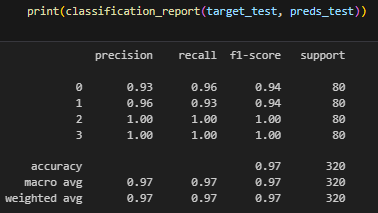
Method 1) Loading the Entire Dataset Result
Method 2) Loading the Batch Dataset Result
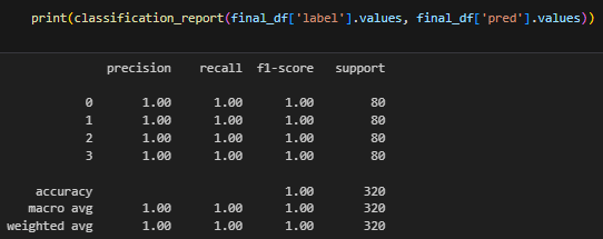
- The F1 score for loading the entire dataset resulted in 0.97, loading the batch dataset resulted in 1.0.
※ Various datasets and tutorial codes can be found in the GitHub repository below.
datahub/dataset/2024 at main · machbase/datahub
All Industrial IoT DataHub with data visualization and AI source - machbase/datahub
 machbase