European Weather Data

This post describes how to use European Weather Data to prediction temperature through AI learning.
Table of Contents
- Data Introduction
- Data Visualization with Machbase Neo
- Table Creation and Data Upload in Machbase Neo
- Experimental Methodology
- Experiment Code
- Experimental Results
1. Data Introduction
- DataHub Serial Number: 2025-2.
- Data Name: European Weather Data.
- Data Collection Methods: The NASA MERRA-2 reanalysis data includes hourly radiation and temperature data for Europe aggregated by Renewables.ninja, with the averages calculated using population-weighted data for each region.
- Data Source: Link
- Raw data size and format: 222MB, CSV.
- Number of tags: 84.
| Tag | Description |
|---|---|
| {code}_radiation_diffuse_horizontal | radiation_diffuse_horizontal weather variable for {code} in W/m2 |
| {code}_radiation_direct_horizontal | radiation_direct_horizontal weather variable for {code} in W/m2 |
| {code}_temperature | temperature weather variable for {code} in degrees C |
| utc_timestamp | Start of time period in Coordinated Universal Time |
| Code | Country |
|---|---|
| AT | Austria |
| BE | Belgium |
| BG | Bulgaria |
| CH | Switzerland |
| CZ | Czech Republic |
| DE | Germany |
| DK | Denmark |
| EE | Estonia |
| ES | Spain |
| FI | Finland |
| FR | France |
| GB | United Kingdom |
| GR | Greece |
| HR | Croatia |
| HU | Hungary |
| IE | Ireland |
| IT | Italy |
| LT | Lithuania |
| LU | Luxembourg |
| LV | Latvia |
| NL | Netherlands |
| NO | Norway |
| PL | Poland |
| PT | Portugal |
| RO | Romania |
| SE | Sweden |
| SI | Slovenia |
| SK | Slovakia |
- Data Time Range: 1980-01-01 00:00:00 to 2020-01-01 00:00:00.
- Number of data records collected: 29,456,760.
- CSV data URL: https://data.yotahub.com/2025-2/datahub-2025-2-EU-weather.csv.gz
- Data Migration: European Weather Data Migration
2. Data Visualization with Machbase Neo
- Data visualization is possible through the Tag Analyzer in Machbase Neo.
- Select desired tag names and visualize them in various types of graphs.
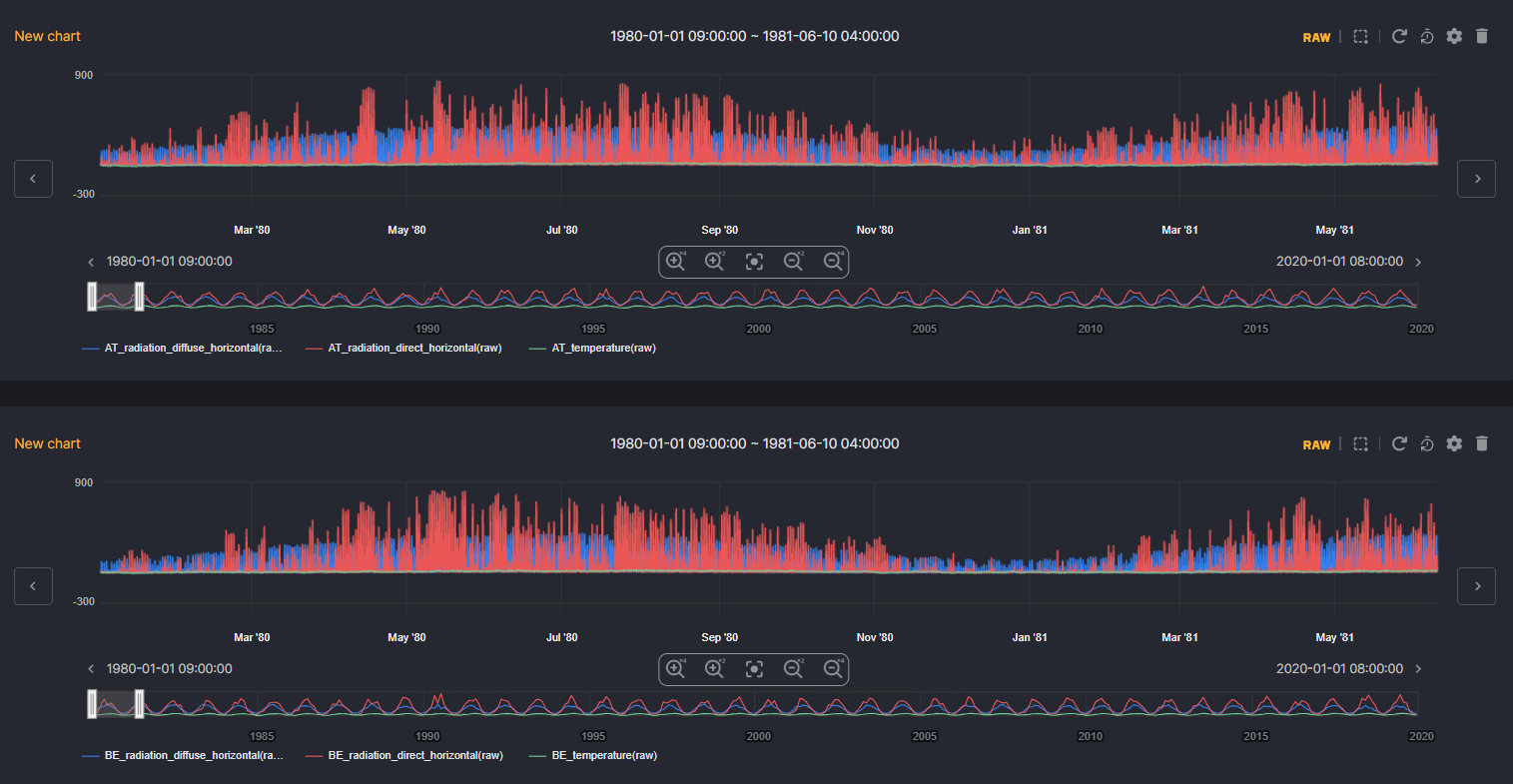
- Below, access the 2025-2 DataHub in real-time, select the desired tag names from the data of 84 tags, visualize them, and preview the data patterns.
DataHub Viewer
3. Table Creation and Data Upload in Machbase Neo
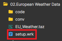
- In the DataHub directory, use setup.wrk located in the European Weather Dataset folder to create tables and load data, as illustrated in the image below.
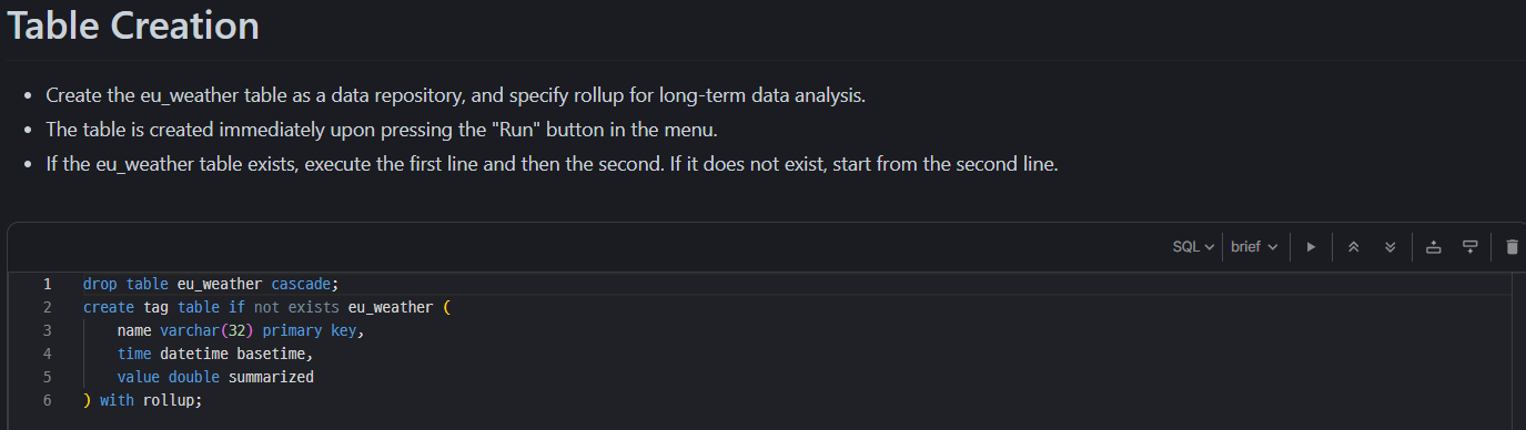
1) Table Creation
- The table is created immediately upon pressing the "Run" button in the menu.
- If the eu_weather table exists, execute the first line and then the second. If it does not exist, start from the second line.
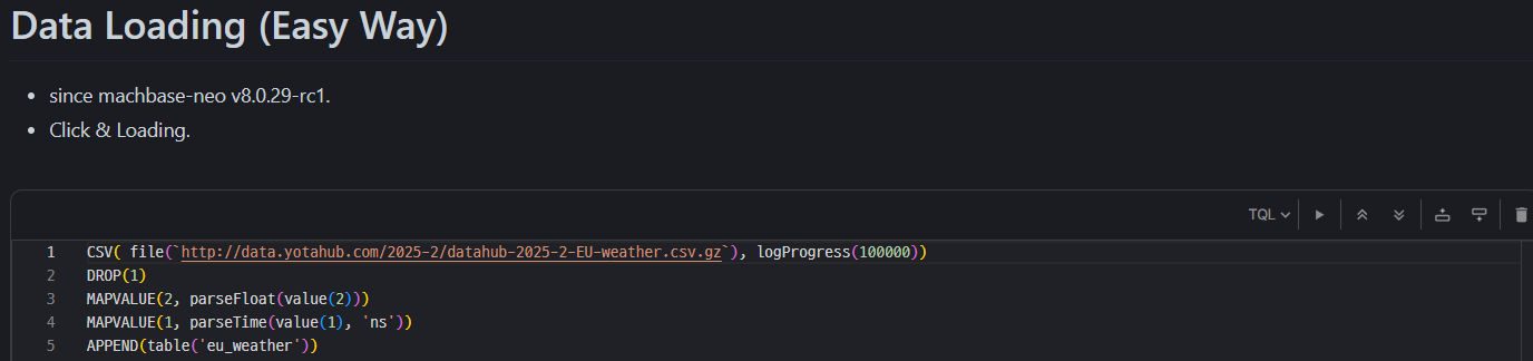
2) Data Upload
- Loading tables in two different ways.
Method 1) Table loading method using TQL in Machbase Neo (since machbase-neo v8.0.29-rc1
-
Pros
- Machbase Neo loads as soon as you hit the launch button.
-
Cons
- Slower table loading speed compared to other method.
Method 2) Loading tables using commands
-
Pros
- Fast table loading speed.
-
Cons
- The table loading process is cumbersome.
- Run cmd window - Change machbase-neo path - Enter command in cmd window.
- If run the below script from the command shell, the data will be entered at high speed into the eu_weather table.
curl http://data.yotahub.com/2025-2/datahub-2025-2-EU-weather.csv.gz | machbase-neo shell import --input - --compress gzip --header --method append --timeformat ns eu_weather
- If specify a separate username and password, use the --user and --password options (if not sys/manager) and add the options as shown below.
curl http://data.yotahub.com/2025-2/datahub-2025-2-EU-weather.csv.gz | machbase-neo shell import --input - --compress gzip --header --method append --timeformat ns eu_weather --user USERNAME --password PASSWORD
4. Experimental Methodology
- Model Objective: Austria Temperature Forecasting.
- Tags Used: AT_temperature.
- Model Configuration: PatchMixer.
- Learning Method: supervised Learning.
- Train: Model Training.
- Test: Model Performance Evaluation Based on Austria Temperature Forecasting.
- Model Optimizer: Adam.
- Model Loss Function: Mean Squared Error.
- Model Performance Metric: Mean Squared Error & R2 Score.
- Data Loading Method
- Loading the Entire Dataset.
- Loading the Fetch Dataset.
- Data Preprocessing
- MinMax Scaling.
5. Experiment Code
- Composed of three methods.
- Data Information: Outputs general information about the data.
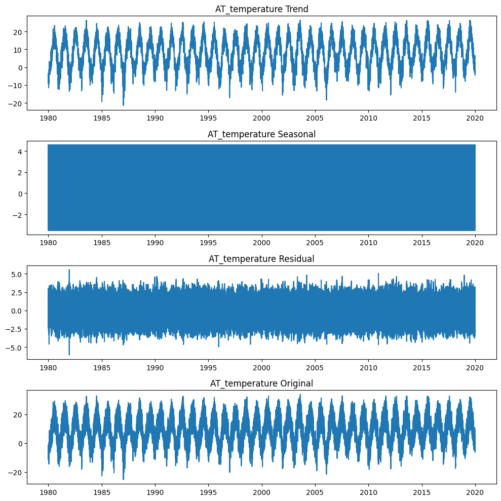
- Visual Information: correlation heatmap, plot, Decomposition about the data.
- Statistical Test: ADF Test, KPSS Test, PP Test, ljung box Test, Arch Test, VIF Test about the data.
- The entire code can be run through 2.European_Weather_EDA.
Austria Temperature Forecasting
- Below is the code for each of the two ways to get data from the database.
- If all the data can be loaded and trained at once without causing memory errors, then method 1 is the fastest and simplest.
- If the data is too large, causing memory errors, then the batch loading method proposed in method 2 is the most efficient.
Method 1) Loading the Entire Dataset
- The code below is implemented in a way that loads all the data needed for training from the database all at once.
- It is exactly the same as loading all CSV files (The only difference is that the data is loaded from Machbase Neo).
- Pros
- Can use the same code that was previously utilizing CSVs (Only the loading process is different).
- Cons
- Unable to train if trainable data size exceeds memory size.
- The entire code can be run through 2.European_Weather_Full.
Method 2) Loading the Fetch Dataset
- Method for loading data from the Machbase Neo for a buffer size.
- Pros
- It is possible to train the model regardless of the data size, no matter how large it is.
- Cons
- It takes longer to train compared to method 1.
- The entire code can be run through 2.European_Weather_Buffered_Fetch.
6. Experimental Results
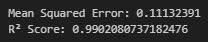
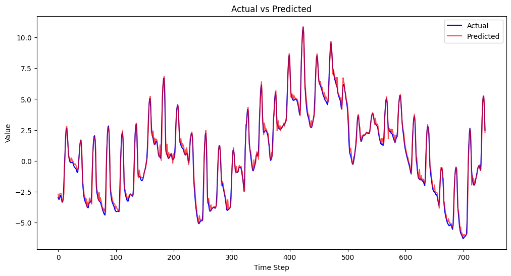
Method 1) Loading the Entire Dataset Result
Method 2) Loading the Fetch Dataset Result
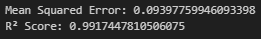
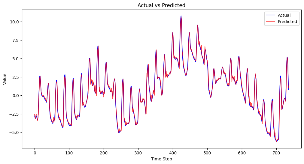
- The R2 score shows high performance above 0.9 in both methods.
- The actual scale-based MSE value is also around 0.1, demonstrating decent performance.
※ Various datasets and tutorial codes can be found in the GitHub repository below.
datahub/dataset at main · machbase/datahub
All Industrial IoT DataHub with data visualization and AI source - machbase/datahub
 machbase