Electricity Transformer Data

This post describes how to train AI using various data (efficiency, temperature, etc.) from a transformer and use the model to forecast data.
Table of Contents
- Data Introduction
- Data Visualization with Machbase Neo
- Table Creation and Data Upload in Machbase Neo
- Experimental Methodology
- Experiment Code
- Experimental Results
1. Data Introduction
- DataHub Serial Number: 2024-6.
- Data Name: Electricity Transformer Data.
- Data Collection Methods: Data was collected from electrical transformers in two regions of China at 15-minute and 1-hour intervals.
- Data Source: Link
- Raw data size and format: 25MB, CSV.
- Number of tags: 28.
- Total of 4 instances each, based on time collection intervals and regions.
| TAG | DESCRIPTION |
|---|---|
| HUFL (High UseFul Load) | A high level of load that is effectively utilized in the power system. |
| HULL (High UseLess Load) | A high level of load that is not efficiently utilized in the power system. |
| MUFL (Middle UseFul Load) | A middle level of load that is effectively utilized in the power system. |
| MULL (Middle UseLess Load) | A middle level of load that is not efficiently utilized in the power system. |
| LUFL (Low UseFul Load) | A low level of load that is effectively utilized in the power system. |
| LULL (Low UseLess Load) | A low level of load that is not efficiently utilized in the power system. |
| OT (Oil Temperature) | The temperature of the oil in the system. |
- Data Time Range: 2016-07-01 00:00:00 to 2018-06-26 19:45:00.
- Number of data records collected: 1,219,400.
- CSV data URL: https://data.yotahub.com/2024-6/datahub-2024-06-elec-transformer.csv.gz
- Data Migration: Electricity Transformer Data Migration
2. Data Visualization with Machbase Neo
- Data visualization is possible through the Tag Analyzer in Machbase Neo.
- Select desired tag names and visualize them in various types of graphs.
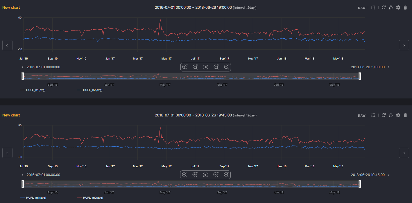
- Below, access the 2024-6 DataHub in real-time, select the desired tag names from the data of 28 tags, visualize them, and preview the data patterns.
DataHub Viewer
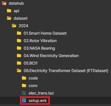
3. Table Creation and Data Upload in Machbase Neo
- In the DataHub directory, use setup.wrk located in the Electricity Transformer Dataset folder to create tables and load data, as illustrated in the image below.
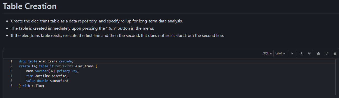
1) Table Creation
- The table is created immediately upon pressing the "Run" button in the menu.
- If the elec_trans table exists, execute the first line and then the second. If it does not exist, start from the second line.
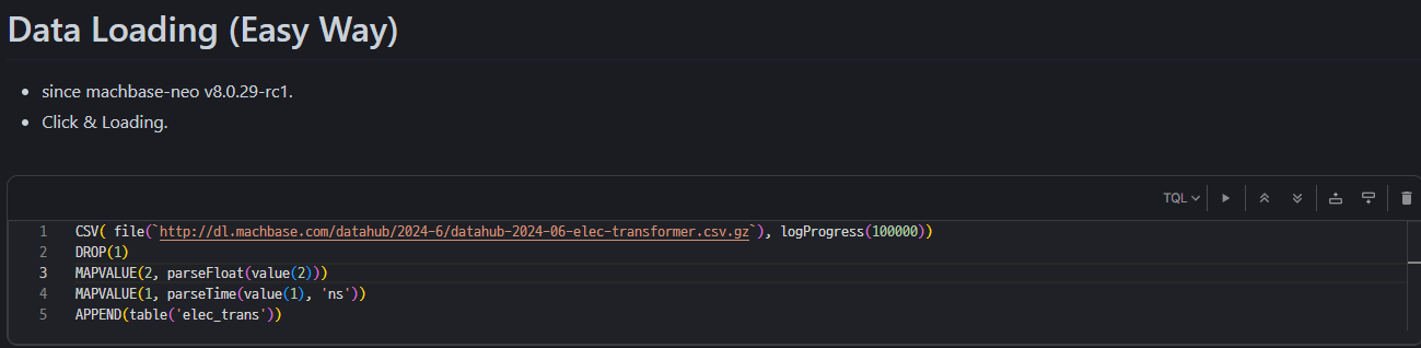
2) Data Upload
- Loading tables in two different ways.
Method 1) Table loading method using TQL in Machbase Neo (since machbase-neo v8.0.29-rc1
-
Pros
- Machbase Neo loads as soon as you hit the launch button.
-
Cons
- Slower table loading speed compared to other method.
Method 2) Loading tables using commands
-
Pros
- Fast table loading speed.
-
Cons
- The table loading process is cumbersome.
- Run cmd window - Change machbase-neo path - Enter command in cmd window.
- If run the below script from the command shell, the data will be entered at high speed into the elec_trans table.
curl http://data.yotahub.com/2024-6/datahub-2024-06-elec-transformer.csv.gz | machbase-neo shell import --input - --compress gzip --header --method append --timeformat ns elec_trans
- If specify a separate username and password, use the --user and --password options (if not sys/manager) and add the options as shown below.
curl http://data.yotahub.com/2024-6/datahub-2024-06-elec-transformer.csv.gz | machbase-neo shell import --input - --compress gzip --header --method append --timeformat ns elec_trans --user USERNAME --password PASSWORD
4. Experimental Methodology
- Model Objective: Oil Temperature Forecasting.
- Tags Used: 1-hour interval data from Region 1 in China.
- Model Configuration: BILSTM.
- Learning Method: Unsupervised Learning.
- Train: Model Training.
- Test: Model Performance Evaluation Based on Oil Temperature Forecasting.
- Model Optimizer: Adam.
- Model Loss Function: Mean Squared Error.
- Model Performance Metric: Mean Squared Error & R2 Score.
- Data Loading Method
- Loading the Entire Dataset.
- Loading the Batch Dataset.
- Data Preprocessing
- Time series decomposition.
- MinMax Scaling.
5. Experiment Code
- Below is the code for each of the two ways to get data from the database.
- If all the data can be loaded and trained at once without causing memory errors, then method 1 is the fastest and simplest.
- If the data is too large, causing memory errors, then the batch loading method proposed in method 2 is the most efficient.
Method 1) Loading the Entire Dataset
- The code below is implemented in a way that loads all the data needed for training from the database all at once.
- It is exactly the same as loading all CSV files (The only difference is that the data is loaded from Machbase Neo).
- Pros
- Can use the same code that was previously utilizing CSVs (Only the loading process is different).
- Cons
- Unable to train if trainable data size exceeds memory size.
- The entire code can be run through 6.Elec_Trans_General.ipynb.
Method 2) Loading the Batch Dataset
- Method for loading data from the Machbase Neo for a single batch size.
- The code below is for fetching a time range sequentially for a single batch size.
- Pros
- It is possible to train the model regardless of the data size, no matter how large it is.
- Cons
- It takes longer to train compared to method 1.
- The entire code can be run through 6.Elec_Trans_New_Batch.ipynb.
6. Experimental Results
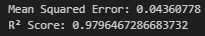
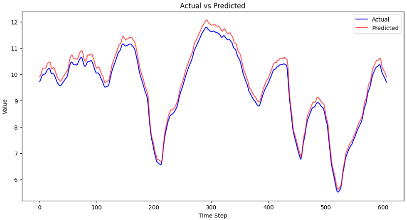
Method 1) Loading the Entire Dataset Result
Method 2) Loading the Batch Dataset Result
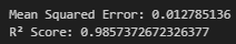
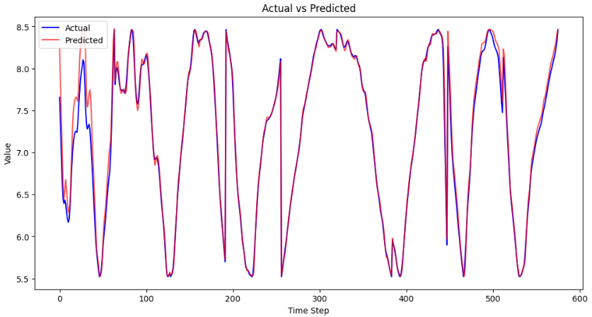
- The R2 score for loading the entire dataset resulted in 0.979, loading the batch dataset resulted in 0.985.
※ Various datasets and tutorial codes can be found in the GitHub repository below.
datahub/dataset/2024 at main · machbase/datahub
All Industrial IoT DataHub with data visualization and AI source - machbase/datahub
 machbase