Appliances Energy Data
This post describes how to perform AI training based on power consumption data from home appliances, indoor temperature and humidity data, and weather data to forecast future data.
Table of Contents
- Data Introduction
- Data Visualization with Machbase Neo
- Table Creation and Data Upload in Machbase Neo
- Experimental Methodology
- Experiment Code
- Experimental Results
1. Data Introduction
- DataHub Serial Number: 2024-9.
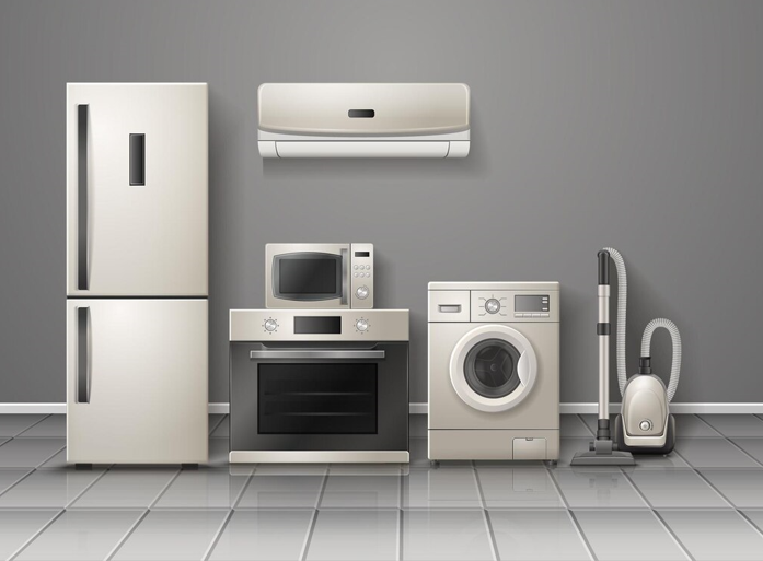
- Data Name: Appliances Energy Data.
- Data Collection Methods: Power usage data of household appliances inside a building was collected at 10-minute intervals for approximately 4.5 months, including temperature and humidity of different parts of the building, as well as internal and external weather data.
- Data Source: Link
- Raw data size and format: 20MB, CSV.
- Number of tags: 29.
| TAG | DESCRIPTION |
|---|---|
| time | Date. |
| Appliances | Power consumption of household appliances (wh). |
| lights | Power consumption of lighting devices (wh). |
| T1 | Temperature in the kitchen (°C). |
| RH_1 | Humidity in the kitchen (%). |
| T2 | Temperature in the living room (°C). |
| RH_2 | Humidity in the living room (%). |
| T3 | Temperature around the laundry room (°C). |
| RH_3 | Humidity in the laundry room (%). |
| T4 | Indoor temperature in the office (°C). |
| RH_4 | Indoor humidity in the office (%). |
| T5 | Temperature in the bathroom (°C). |
| RH_5 | Humidity in the bathroom (%). |
| T6 | Temperature outside the building (north side) (°C). |
| RH_6 | Humidity outside the building (north side) (%). |
| T7 | Temperature in the ironing room (°C). |
| RH_7 | Humidity in the ironing room (%). |
| T8 | Temperature in the second teenage room (°C). |
| RH_8 | Humidity in the second teenage room (%). |
| T9 | Temperature in the master bedroom (°C). |
| RH_9 | Humidity in the master bedroom (%). |
| T_out | Outdoor temperature according to Chievres weather station (°C). |
| Press_mm_hg | Atmospheric pressure according to Chievres weather station (mm Hg). |
| RH_out | Outdoor humidity according to Chievres weather station (%). |
| Windspeed | Wind speed according to Chievres weather station (m/s). |
| Visibility | Visibility according to Chievres weather station (km). |
| Tdewpoint | Dew point according to Chievres weather station (°C). |
| rv1 | Random variable 1 (Purpose of preventing overfitting). |
| rv2 | Random variable 2 (Purpose of preventing overfitting). |
- Data Time Range: 2016-01-11 17:00:00 to 2016-05-27 18:00:00.
- Number of data records collected: 552,580.
- CSV data URL: https://data.yotahub.com/2024-9/datahub-2024-09-Appliances-Energy.csv.gz
- Data Migration: Appliances Energy Data Migration
2. Data Visualization with Machbase Neo
- Data visualization is possible through the Tag Analyzer in Machbase Neo.
- Select desired tag names and visualize them in various types of graphs.
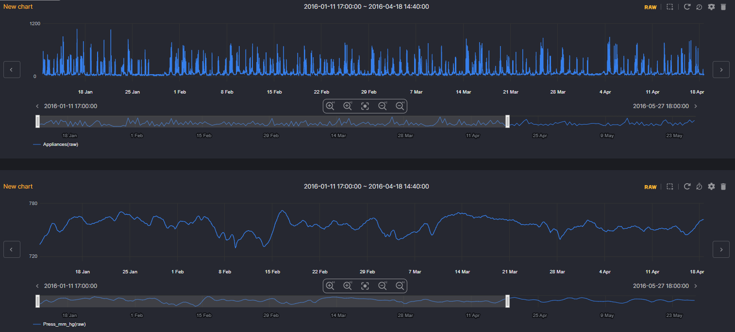
- Below, access the 2024-9 DataHub in real-time, select the desired tag names from the data of 29 tags, visualize them, and preview the data patterns.
DataHub Viewer
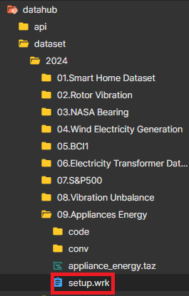
3. Table Creation and Data Upload in Machbase Neo
- In the DataHub directory, use setup.wrk located in the Appliances Energy Dataset folder to create tables and load data, as illustrated in the image below.
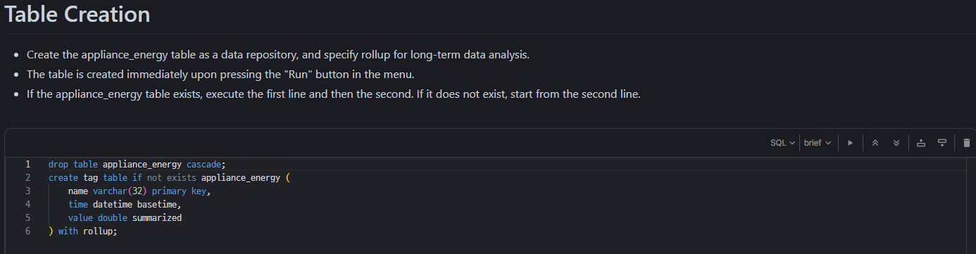
1) Table Creation
- The table is created immediately upon pressing the "Run" button in the menu.
- If the appliance_energy table exists, execute the first line and then the second. If it does not exist, start from the second line.
2) Data Upload
- Loading tables in two different ways.
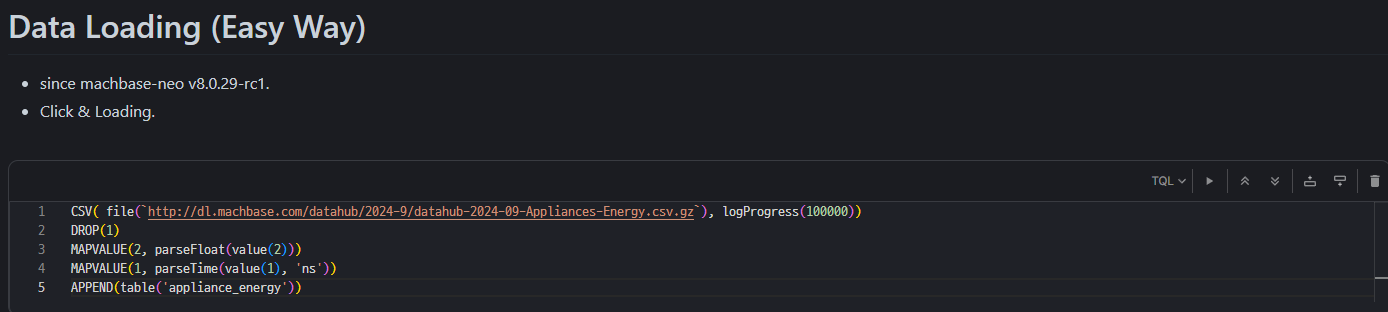
Method 1) Table loading method using TQL in Machbase Neo (since machbase-neo v8.0.29-rc1
-
Pros
- Machbase Neo loads as soon as you hit the launch button.
-
Cons
- Slower table loading speed compared to other method.
Method 2) Loading tables using commands
-
Pros
- Fast table loading speed.
-
Cons
- The table loading process is cumbersome.
- Run cmd window - Change machbase-neo path - Enter command in cmd window.
- If run the below script from the command shell, the data will be entered at high speed into the appliance_energy table.
curl http://data.yotahub.com/2024-9/datahub-2024-09-Appliances-Energy.csv.gz | machbase-neo shell import --input - --compress gzip --header --method append --timeformat ns appliance_energy
- If specify a separate username and password, use the --user and --password options (if not sys/manager) and add the options as shown below.
curl http://data.yotahub.com/2024-9/datahub-2024-09-Appliances-Energy.csv.gz | machbase-neo shell import --input - --compress gzip --header --method append --timeformat ns appliance_energy --user USERNAME --password PASSWORD
4. Experimental Methodology
- Model Objective: Appliances Energy Forecasting.
- Tags Used: all tag name.
- Model Configuration: BILSTM.
- Learning Method: Unsupervised Learning.
- Train: Model Training.
- Test: Model Performance Evaluation Based on Appliances Energy Forecasting.
- Model Optimizer: Adam.
- Model Loss Function: Mean Squared Error.
- Model Performance Metric: Mean Squared Error & R2 Score.
- Data Loading Method
- Loading the Entire Dataset.
- Loading the Batch Dataset.
- Data Preprocessing
- Time series decomposition.
- MinMax Scaling.
- Principal Component Analysis.
5. Experiment Code
- Below is the code for each of the two ways to get data from the database.
- If all the data can be loaded and trained at once without causing memory errors, then method 1 is the fastest and simplest.
- If the data is too large, causing memory errors, then the batch loading method proposed in method 2 is the most efficient.
Method 1) Loading the Entire Dataset
- The code below is implemented in a way that loads all the data needed for training from the database all at once.
- It is exactly the same as loading all CSV files (The only difference is that the data is loaded from Machbase Neo).
- Pros
- Can use the same code that was previously utilizing CSVs (Only the loading process is different).
- Cons
- Unable to train if trainable data size exceeds memory size.
- The entire code can be run through 6.Appliances_Energy_Full.ipynb.
Method 2) Loading the Batch Dataset
- Method for loading data from the Machbase Neo for a single batch size.
- The code below is for fetching a time range sequentially for a single batch size.
- Pros
- It is possible to train the model regardless of the data size, no matter how large it is.
- Cons
- It takes longer to train compared to method 1.
- The entire code can be run through 6.Appliances_Energy_Buffered_Fetch.ipynb.
6. Experimental Results
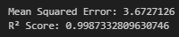
Method 1) Loading the Entire Dataset Result
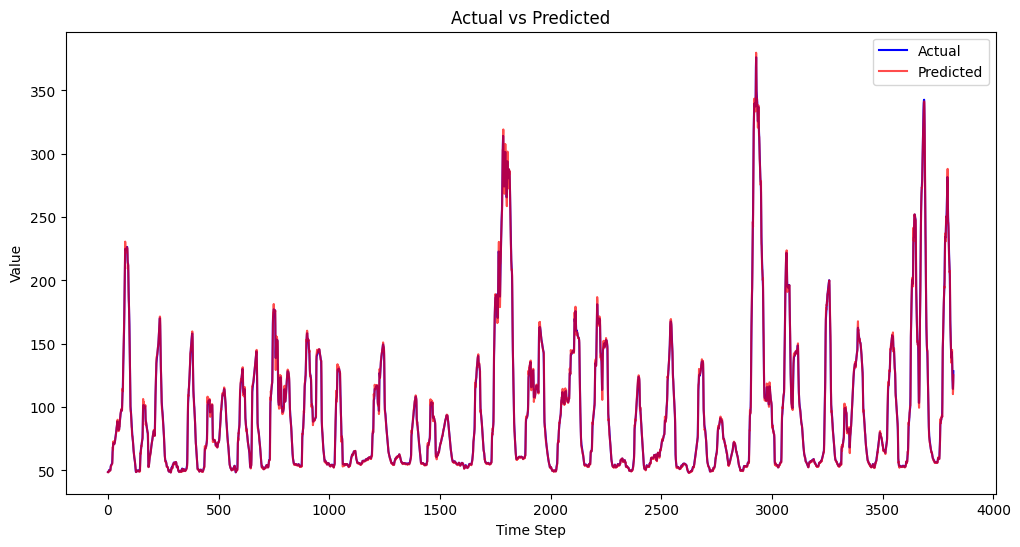
Method 2) Loading the Batch Dataset Result
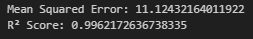
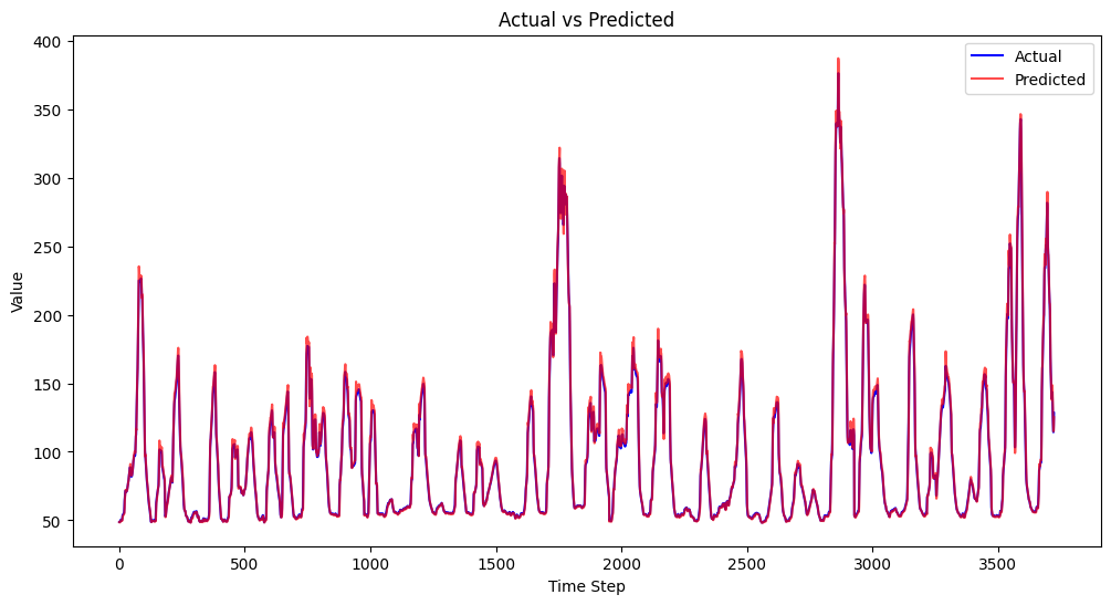
- The R2 score for loading the entire dataset resulted in 0.95, loading the batch dataset resulted in 0.99.
※ Various datasets and tutorial codes can be found in the GitHub repository below.
datahub/dataset at main · machbase/datahub
All Industrial IoT DataHub with data visualization and AI source - machbase/datahub
 machbase